IDC6940

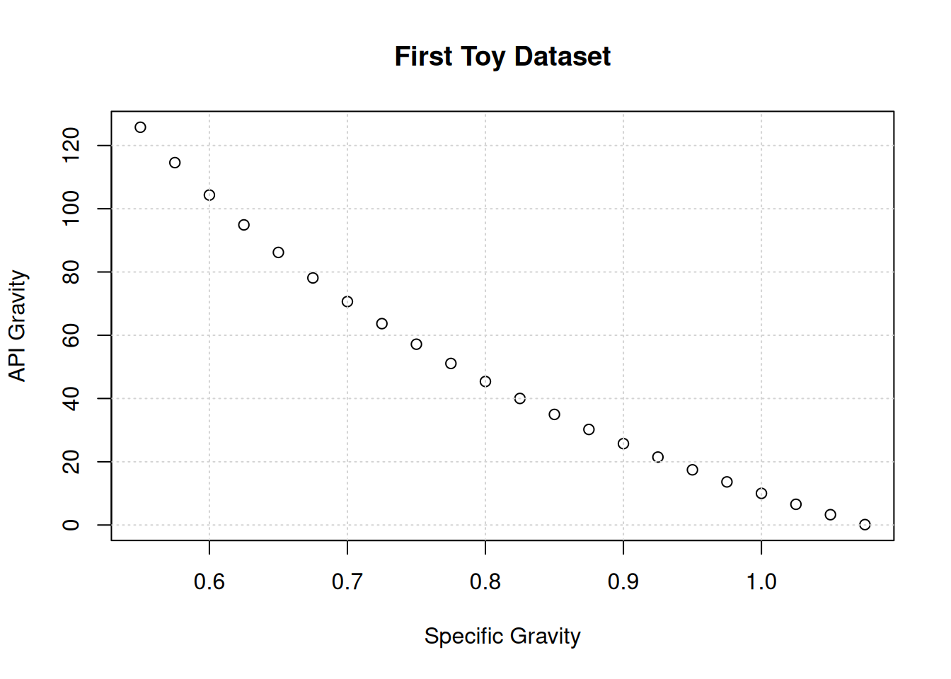
Weekly Report 4

Let’s start by rebuilding our toy data set:

\(\gamma_{api}=\frac{141.5}{\gamma_o}-131.5\)

x <- seq(from=0.55, to=1.075, by=0.025)
y <- 141.5/x-131.5
plot(x,y,main="First Toy Dataset",xlab="Specific Gravity",ylab="API Gravity")
grid()

Alternating Conditional Expectations

This is a technology can be viewed as a cross between the Box-Cox transform and Linear Regression. The idea is to improve the fit of the straight line by iteratively transforming both the dependent and the independent variables.

Let’s continue by importing our library:

library("acepack")

Next, we fit the data:

myMod<-ace(x,y)

Now we can examine the relationship between the transformed variables:

plot(myMod$tx,myMod$ty,main="First Toy Dataset",xlab="Transformed Specific Gravity",ylab="Transformed API Gravity")
grid()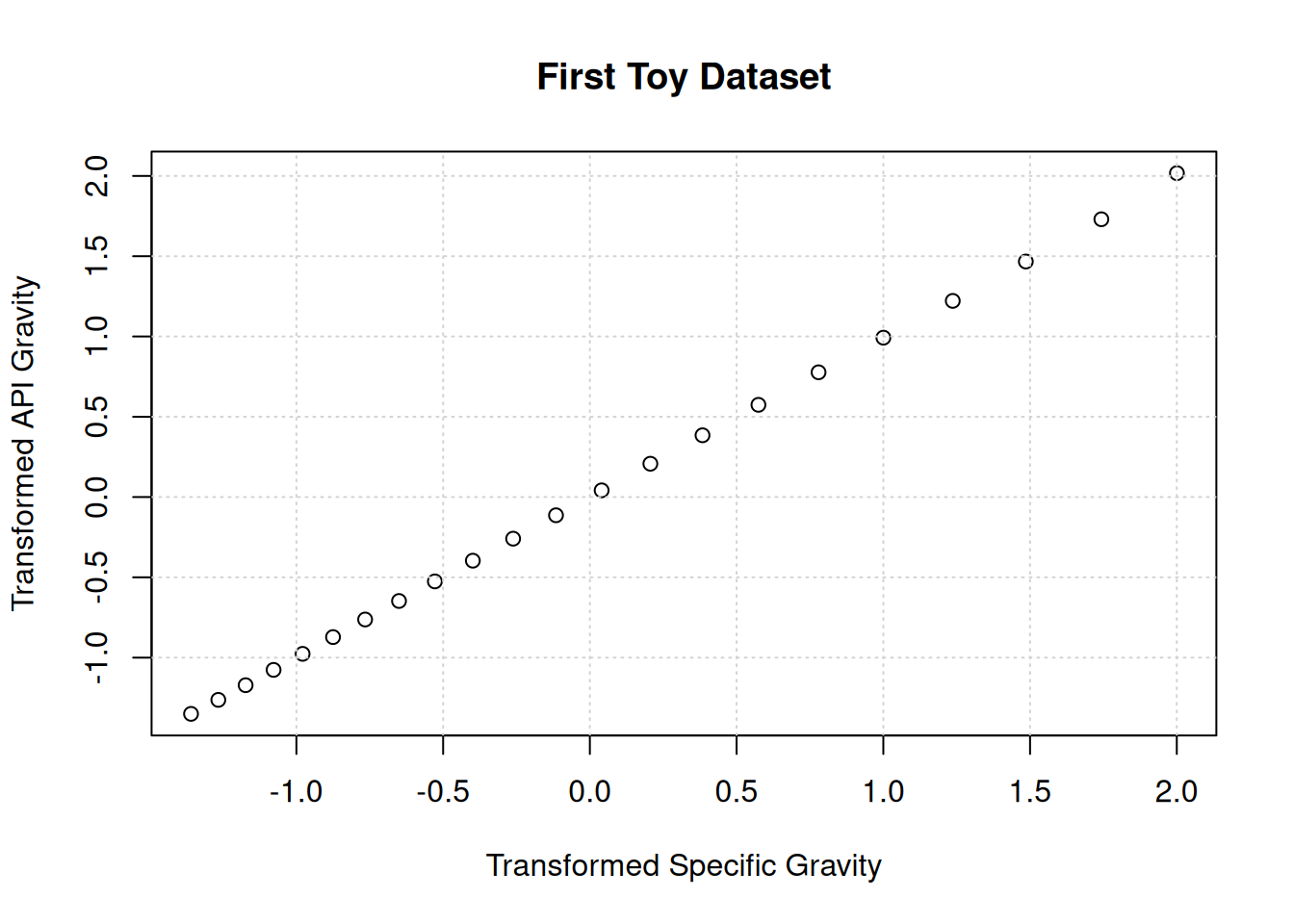

As expected, the algorithm finds a straight-line relationship. However, the change in slope direction (negative to positive) is a surprise!

Let us look at the independent variable transformation:

plot(x,myMod$tx,main="First Toy Dataset",xlab="Specific Gravity",ylab="Transformed Specific Gravity")
grid()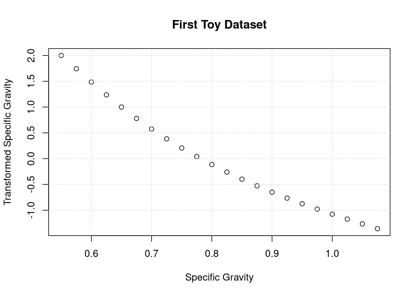

And now the dependent variable:

plot(y,myMod$ty,main="First Toy Dataset",xlab="API Gravity",ylab="Transformed API Gravity")
grid()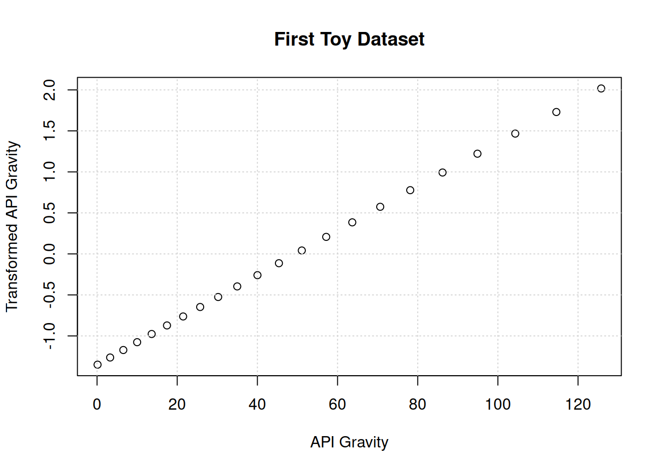

This relationship appears to be linear, and looks as though it is shifted.

Tentative Conclusions

1. The method works
2. We need to figure out how to extract the transformations. In the worst-case scenario, we can use symbolic regression…